Getting Started
We start directly with a tutorial of a very simple Optimal Control Problem (OCP).
The basic features of moba_muscod are explained in conjunction with an introduction
to OCP formulation. More advanced tutorials can be found following the links below.
moba_muscod uses object-oriented representations of OCPs. The main class is
OptimalControlProblem. The first step is to create an instance of this class:
import moba_muscod as momu
ocp = momu.OptimalControlProblem()
Now this object represents our specific Optimal Control Problem. An high-level user interface for the most common settings can be used by calling member function of this object. Expert users could also directly access low-level elements.
The most important part of an OCP is are differential equations that describe the dynamics of the considered system. We use the open and standarized Functional Mock-up Interface to provide differential equations. The model can be exported from any simulation tool that supports FMI for Model Exchange 2.0. See FMI website for a list of available tools.
In our case the system dynamics are given by the simple first order differential equation

This model is loaded as Functional Mock-up Unit (FMU):
ocp.loadFMU('FirstOrder.fmu')
The model contains Parameters. By default they are all included as optimization variables. In this example we don’t want to have any parameter free for optimization:
ocp.selectParameters([])
Finally, we want to find the optimal trajectory for the input u on a fixed time horizon of 5 seconds. In order to make the problem numerical computable, we discretize the trajectory piecewise constant on an equidistant time grid of 20 intervals:
ocp.setTimeHorizon(nmsi=20, hstart=5.0)
Please note, that we use the Direct Multiple Shooting Method, where the differential states are also discretized on the same grid.
The next step is to define, what we mean by saying “optimal”. The so called cost function returns a scalar value, that needs to be minimized. We want to minimize the squared deviation of the state x from a set-point of 1.0. By using a Lagrange-type term we define, that the given expression should be integrated over the whole time horizon:
ocp.setCostFunction(lval = '(x0-1.0)*(x0-1.0)')
We provide initial values for state x and control u:
ocp.setInitialValues(xInit=[-1.0], uInit=[2.0])
With default settings this means, that x is fixed to the given initial value at the beginning of the time horizon: ..math:
x(t=0) = -1.0
Whereas the controls are not fixed at all. The given initial value is used as starting guess for the iterative optimization. In the end we want to get optimal values for the control in each interval as result. We need to provide lower and upper bounds for x und u:
ocp.setLowerBounds(xBounds=[-2.1], uBounds=[-2.0])
ocp.setUpperBounds(xBounds=[ 2.1], uBounds=[ 2.0])
These bounds are constraints, which have to be strictly fulfilled at the optimization result. They hold for the whole time horizon.
We also want to add an equality constraint for u at the start time:
ocp.addConstraint('u0=-2.0', 's')
Now, our OCP is mathematically completely defined. But as it is true for all kind of numerical optimization, we need to carefully select scaling values for all variables, in order to get the algorithm working smoothly. This is done with:
ocp.setScaleValues(xScale=[1.0], uScale=[1.0], cScale=[0.01])
We finally start the optimization
ocp.solve()
and after successful convergence of the algorithm we plot the result in Python
ocp.plotResult()
or export it into different file formats
ocp.exportResultToModelica()
ocp.exportResultToMatlab()
The plot should look like this:
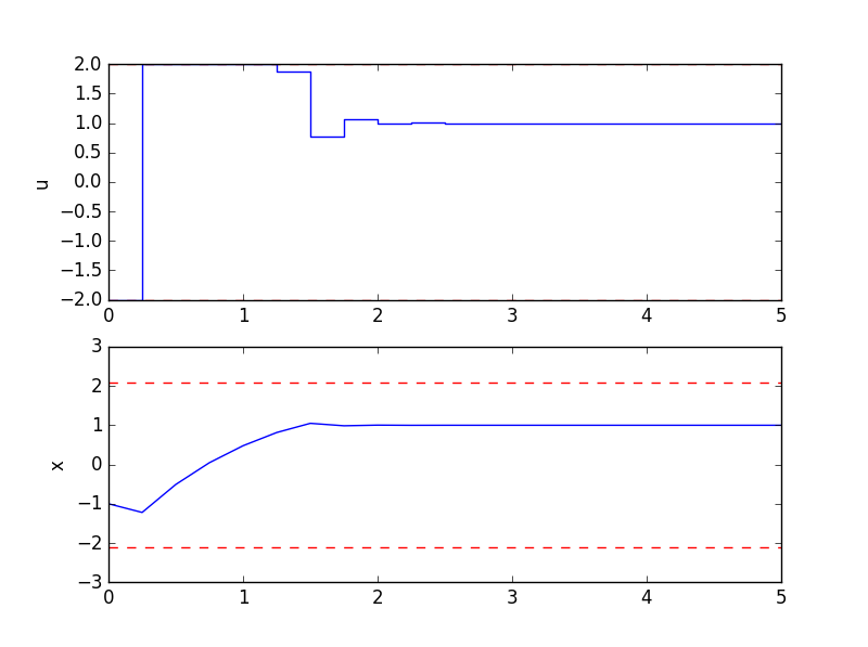
At the first interval the control is at -2.0, as we wanted it by setting the additional equality constraint. After that the control drives the state as fast as possible to its set-point, and keeps it there.
